The Two-Tower Model, Minus the Training

Shoppin was a fashion discovery app: a vertical feed of videos, images, and products that had to feel personal from the first scroll. The catalog was 100,000+ videos and a far larger pool of product and inspiration images, changing daily as we scraped and generated more. This is the problem every discovery feed has on day one: you need a per-user ranking over a corpus too large to score item by item, and at the start you have almost no behavioural data to learn it from. The textbook answer to the first half is a two-tower model; the answer to the second half is to train it on your click log. We had the first problem and not the click log, and shipped anyway. Here is how, and why skipping the training was the right call.

What a two-tower model actually is #

A two-tower model (also called a dual encoder, bi-encoder, or factorized model) is two neural networks that never touch until the very end. One tower, the user or query tower, reads everything you know about the user (history, context, intent) and produces a single vector. The other tower, the item tower, reads an item's features and produces a vector in the same space. Relevance between a user and an item is just the dot product of their two vectors. That is the whole scoring function: one multiply-and-sum in a shared embedding space.

The reason it is drawn as two separate towers, rather than one network that eats a user and an item together, is the entire point of the design. Because the item vector depends only on item features and never on the user, you can compute every item embedding once, offline, and drop them into an approximate-nearest-neighbour (ANN) index. At request time you only run the user tower (one forward pass), get one vector, and ask the index for its top-k nearest items. Cost per request is one small model call plus one sublinear index lookup, no matter whether the corpus is 100,000 items or a billion. A model that fused user and item together would be more expressive, but it would force a forward pass per candidate, which is a non-starter for retrieval.

How you would normally train one #

The canonical way to train the two towers is to treat retrieval as an enormous classification problem: given a user, predict the one item they engaged with out of the entire catalog. You cannot compute a softmax over millions of items per step, so you approximate it with in-batch negatives. For each (user, item-they-liked) pair in a mini-batch, every other item in the same batch is treated as a negative example. It is cheap because those item embeddings are already computed for the batch, and it gives you a dense contrastive signal for free.

L(i) = -log( exp(s(x_i, y_i)/T) / sum_j exp(s(x_i, y_j)/T) )

  s(x, y) = <u(x), v(y)>     # dot product in the shared space
  T                          # temperature, scales the logits

# logQ correction: popular items appear as in-batch negatives too
# often, so subtract their sampling log-probability before softmax:
  s'(x, y) = s(x, y) - log Q(y)

The subtle part is that in-batch negatives are drawn from your traffic, which is a power law, so popular items get sampled as negatives constantly and the model over-penalises them. The fix, from Google's 2019 paper (the one people mean by "the two-tower paper"), is a logQ correction: estimate each item's sampling frequency and subtract its log-probability from the score before the softmax. Then you tune temperature, add uniform negatives so the long tail is reachable, mine a few hard negatives, and keep training and serving features identical so the model does not rot on train-serve skew. It works, and it is a real project.

None of that pays off if you do not yet have the labels. Early on, our engagement data was thin, biased toward whatever we happened to be showing, and changing weekly as the product changed. Training a user tower on it would have baked in that bias and given us a model to babysit (retraining, drift, skew, index-version syncing) at exactly the moment we most needed to iterate on the product. So we made a different bet.

Our version: freeze both towers #

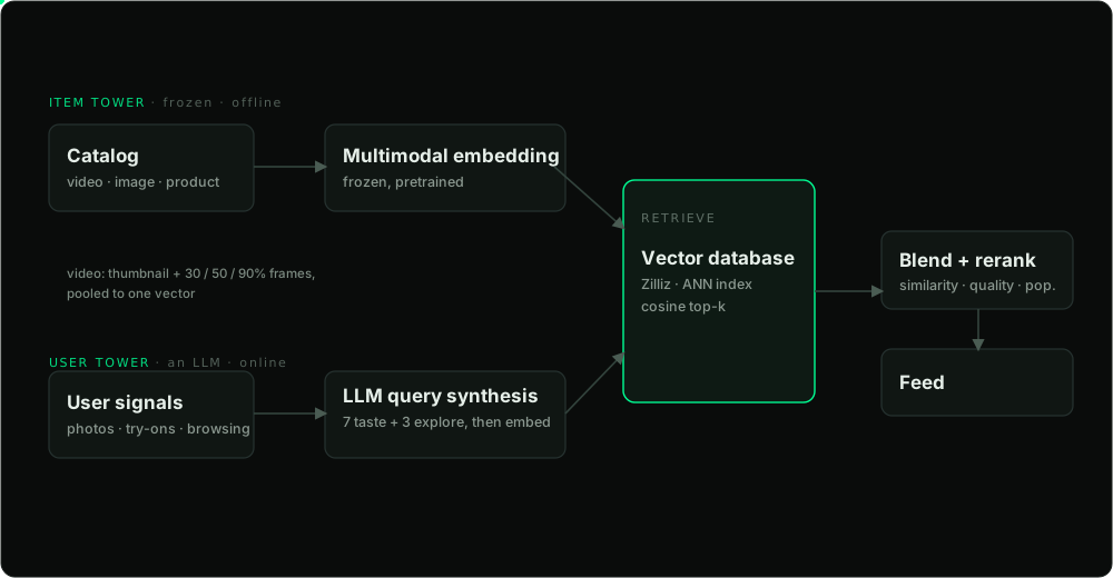
Keep the two-tower architecture (decouple, precompute, ANN) and throw out the training. The item tower becomes a pretrained embedding model we never fine-tune. The user tower becomes something stranger: a large language model that reasons about the user and emits queries, which we then embed with the same encoder. Two encoders, a shared space, a dot product, an index. Dual-encoder-shaped in every way that matters for serving, with zero models trained for retrieval.

The item tower is a pretrained embedding pipeline #

Every inspiration image and product image runs through a pretrained multimodal embedding model that maps a picture straight into a shared vector space. Using a multimodal encoder (we used Gemini's multimodal embeddings) is the load-bearing choice here: because the same model embeds images and text into the same space, a phrase like "cropped leather jacket, muted tones" can be compared directly against a photo with a plain dot product, no separate text and image indexes to reconcile. A distributed pipeline does the unglamorous part: walk the catalog, embed in batches, upsert the vectors in bulk, and run a reconciliation job that keeps the vector store honest against the source of truth. Images and products follow the same path into different collections, and the retrieval mechanics never change. Video is where it gets interesting, because a video is not a picture.

The embedding is not the whole story for an item. Alongside each vector we keep a handful of scalar labels produced by separate classifiers and by Gemini: an aesthetic score, a gender tag, and a set of quality signals (watermarking, composition, safety, an AI-generation likelihood). None of these are learned by a retrieval model. They ride along with the item and get used later, at filter and rerank time, to keep the feed clean and on brand. There is no learned clustering or taxonomy of items; the structure comes entirely from the embedding space plus these labels.

Freezing has one quietly large payoff: there is no train-serve skew, the classic production-ML bug where your offline training features drift from what you compute at request time, because there is no training and the same model produces and serves every embedding. What you trade for it is staleness, embeddings aging as the catalog grows and the encoder version moves, which the reconciliation job and periodic re-embedding handle. Staleness is a far easier thing to reason about than skew.

A video is not one frame #

You cannot embed a fifteen-second clip by embedding its thumbnail and calling it done. A thumbnail is marketing: it is picked to make you tap, and it routinely oversells or plain misrepresents what the clip is actually about. But you also cannot embed every frame, because that is hundreds of near-identical vectors per clip, mostly redundant, and it bloats both the index and the bill. So we sampled the timeline. For each video we took the thumbnail plus the frames at roughly the 30th, 50th, and 90th percentiles of its duration, embedded each of those with the same multimodal model, and pooled them into a single vector. The thumbnail says how the clip presents itself; the percentile frames say how it actually unfolds, including the payoff near the end that a cover frame never shows. One clip becomes one point in the space, and that point represents the whole thing instead of its most clickable instant. Keeping it one point per item, rather than indexing all four frames, is deliberate: the nearest-neighbour math stays a plain top-k, and no clip can out-rank the field just by occupying four slots.

Why a vector database earns its place #

Once every item is a vector, you have to decide where those vectors live and how you search them. The naive option is to keep them in your primary database and compute cosine similarity in a query, and for a few thousand rows that is genuinely fine. At a hundred thousand videos and a far larger pool of images it falls over, because exact nearest-neighbour search is linear in the corpus: every request reads every vector. That is a full scan on the hot path of your feed, on every scroll, for every user. A vector database exists to make that sublinear. It builds an approximate-nearest-neighbour index so a top-k lookup touches a small fraction of the corpus, it lets you attach scalar fields (gender, quality flags, freshness) and filter on them inside the same search, and it owns the operational work (sharding, replication, streaming upserts as the catalog changes) that you do not want to hand-roll. We used Zilliz, the managed form of Milvus, precisely so the index and the ops were somebody else's problem and our attention could go to retrieval and ranking.

The user tower is a language model #

This is the part I like most. Instead of a learned user encoder, the user tower is a two-stage Gemini pipeline. Stage one reads the user's visual context: their own photos, up to five recent virtual-try-on results, and up to five images they have been browsing, and summarises appearance, colour and silhouette preferences, and a few style vibes. Stage two takes that summary plus engagement signals (which past queries they actually interacted with, weighted real searches versus onboarding-derived vibes, Pinterest board names) and produces exactly ten short search queries.

Those ten queries are not random. The prompt mandates the split explicitly: seven that extend the user's current taste, and three from adjacent aesthetics they have not explored yet. Each query is then embedded with the same 1536-dimensional encoder the items use, and the resulting vectors are mean-pooled and L2-normalised into a single query vector. That vector goes into the ANN index exactly as a trained user tower's output would. The difference is that ours is a sentence first and a vector second.

Framing the user tower as an LLM buys three things a trained encoder would have made hard. Cold start mostly disappears: the model can reason from a single profile photo and a few browse images, so a brand-new user still gets a coherent feed. The feed is explainable, because the intermediate representation is human-readable queries you can log and eyeball, not an opaque 1536-dim point. And the explore-versus-exploit balance is a line in a prompt (seven taste, three adjacent) a product person can reason about, not a hyperparameter you move by retraining. Demographics ride along the same way: age and body type as a natural-language suffix on the query, ethnicity as context in the prompt, never a hard filter on the vectors.

Retrieval, then a stack of heuristics #

Serving is an ANN top-k over cosine similarity. Two details matter. First, the set of items the user has already seen is excluded inside the vector search's own filter, at retrieval time, not after, so you never waste the top-k on things you are about to drop. Second, you can lean on the database's range search to grab a band of results that are similar but not near-identical, which is how you get variety without the feed collapsing into ten shots of the same jacket.

near-duplicate   cosine >= 0.90    drop, it is the same look
core match       cosine >= 0.75    keep, rank it high
usable           cosine >= 0.20    keep as filler / explore
below floor      cosine <  0.20    discard

result dedup     two results too close -> drop one
range band       ~0.75 to 0.90     "similar, not a dupe"

Whatever survives retrieval is reranked by a blend, not by cosine alone. Similarity gets you relevance; the other terms get you quality and freshness. An aesthetic score pulls prettier results up, a click-through-rate percentile (computed within the batch so it is scale-free) rewards things that actually perform, and raw popularity is best handled by sampling rather than a fixed weight, so a single viral item does not pin itself to the top forever. Recency decays with a short half-life, and a per-user cursor walks through the user's queries across requests so consecutive scrolls do not keep serving the same seed.

score =  0.8 * cosine
       + 0.2 * (aesthetic_score / 100)     # quality signal, 0..100
       + 0.3 * ctr_rank_percentile          # within-batch, scale-free

# popularity is sampled, not a fixed term: draw from a Beta
# posterior on each item's engagement (Thompson sampling), with a
# per-query cap so one viral query cannot flood the row. Different
# engagements weigh differently: an order counts for more than a view.

Explore vs exploit, without a bandit you have to train #

How much of the feed is personalised (drawn from the user's own query vectors) versus explore or viral content is decided per user by a single function over a composite activity signal. Query volume weighs more than raw clicks, blended with how recently the user has been active, and the result maps to a personalised share somewhere between about 20% and 80%, sitting around 60% for a typical user. A user with no queries yet gets an all-explore feed, because there is nothing to personalise on. On top of that sit a few diversity modes that decide how the explore slots split across the user's own affinity, look-alike affinities, and genuinely adjacent ones.

activity        = weighted blend of query volume, clicks, recency
personalised    = clamp(map(activity), ~0.20, ~0.80)   # ~0.60 typical
no queries yet  ->  100% explore       # nothing to personalise on

diversity modes (explore slots: self / look-alike / adjacent):
  self-heavy    3 / 1 / 1
  balanced      2 / 2 / 1
  explore       1 / 2 / 2

A trained system would learn this trade-off from data, most likely as a bandit balancing exploration against exploitation. Ours is a handful of readable constants. That is objectively less clever, and it is also debuggable at 2am, tunable per market without a training run, and impossible to poison with a bad week of data. For the stage we were at, that was the correct trade.

What we gave up by not training #

This is not a free lunch, and pretending otherwise is how you end up defending a system you do not understand. The biggest thing we gave up is learned personalisation inside the embedding itself. A pretrained encoder places two jackets near each other because they look alike, not because this particular user keeps engaging with that specific niche despite a middling visual similarity. A trained user tower can learn that; ours cannot, and we paper over it with the reranking heuristics and the LLM's taste summary.

When you should actually train the towers #

The honest upgrade path is clear. Once you have a real engagement log, one that is large enough and not hopelessly biased by the current feed, training a user tower on it earns you the personalisation the frozen version structurally cannot express. That is the moment to bring back everything from the middle of this post: in-batch negatives with a logQ correction, a few mined hard negatives, careful temperature tuning, and strict train-serve feature parity. You keep the exact same serving shape (precompute item vectors, index them, run one tower at request time), so it is an upgrade to the towers, not a rewrite of the system.

Decoupling the user and item encoders, so the catalog can be precomputed and served from an ANN index, is what makes web-scale retrieval possible, and you get that benefit whether the towers are trained on a billion clicks or frozen off the shelf.

Further reading #

• ▸Yi et al., 2019, Sampling-Bias-Corrected Neural Modeling for Large Corpus Item Recommendations (RecSys). The two-tower paper: in-batch negatives, the logQ correction, and the streaming frequency estimator.
• ▸Covington et al., 2016, Deep Neural Networks for YouTube Recommendations (RecSys). Where the retrieval-then-ranking funnel and serving-via-ANN became standard.
• ▸Huang et al., 2020, Embedding-based Retrieval in Facebook Search (KDD). The hard-negative-mining lessons: hard negatives only cut recall by more than half; you want mostly easy plus a few hard.
• ▸Yang et al., 2020, Mixed Negative Sampling for Learning Two-Tower Neural Networks (WWW). Why in-batch negatives alone never reach the long tail.
• ▸TensorFlow Recommenders (tfrs.tasks.Retrieval, FactorizedTopK, the ScaNN serving layer) if you want the trained version in code.